how do the speeds v1 and v2 compare to v0? that is, what are the ratios v1 v0 and v2 v0 ?

The Kinetic Theory of Gases

12 Distribution of Molecular Speeds

Learning Objectives

By the cease of this section, you will be able to:

Describe the distribution of molecular speeds in an ideal gas
Detect the average and most probable molecular speeds in an platonic gas

Particles in an ideal gas all travel at relatively high speeds, but they do not travel at the same speed. The rms speed is one kind of average, but many particles move faster and many move slower. The actual distribution of speeds has several interesting implications for other areas of physics, as we will see in later chapters.

The Maxwell-Boltzmann Distribution

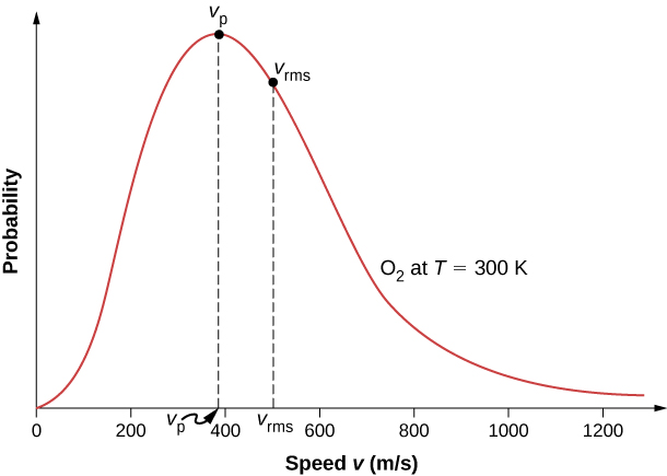
The move of molecules in a gas is random in magnitude and direction for individual molecules, but a gas of many molecules has a predictable distribution of molecular speeds. This predictable distribution of molecular speeds is known as the Maxwell-Boltzmann distribution, after its originators, who calculated information technology based on kinetic theory, and it has since been confirmed experimentally ((Figure)).

To understand this figure, we must define a distribution part of molecular speeds, since with a finite number of molecules, the probability that a molecule will have exactly a given speed is 0.

The Maxwell-Boltzmann distribution of molecular speeds in an ideal gas. The near likely speed ${v}_{\text{p}}$ is less than the rms speed ${v}_{\text{rms}}$ . Although very high speeds are possible, only a tiny fraction of the molecules have speeds that are an order of magnitude greater than ${v}_{\text{rms}}.$

We ascertain the distribution function $f\left(v\right)$ by saying that the expected number $N\left({v}_{1},{v}_{2}\right)$ of particles with speeds between ${v}_{1}$ and ${v}_{2}$ is given by

$N\left({v}_{1},{v}_{2}\right)=N{\int }_{{v}_{1}}^{{v}_{2}}\phantom{\rule{0.2em}{0ex}}f\left(v\right)dv.$

[Since N is dimensionless, the unit of f(v) is seconds per meter.] Nosotros tin can write this equation conveniently in differential form:

$dN=Nf\left(v\right)dv.$

In this grade, nosotros can understand the equation as saying that the number of molecules with speeds between 5 and $v+dv$ is the full number of molecules in the sample times f(v) times dv. That is, the probability that a molecule's speed is betwixt v and $v+dv$ is f(v)dv.

Nosotros tin now quote Maxwell'due south result, although the proof is beyond our scope.

Maxwell-Boltzmann Distribution of Speeds

The distribution part for speeds of particles in an ideal gas at temperature T is

$f\left(v\right)=\frac{4}{\sqrt{\pi }}{\left(\frac{m}{2{k}_{\text{B}}T}\right)}^{3\text{/}2}\phantom{\rule{0.2em}{0ex}}{v}^{2}{e}^{\text{−}m{v}^{2}\text{/}2{k}_{\text{B}}T}.$

The factors before the ${v}^{2}$ are a normalization constant; they make sure that $N\left(0,\infty \right)=N$ by making sure that ${\int }_{0}^{\infty }\phantom{\rule{0.2em}{0ex}}f\left(v\right)dv=1.$ Let'southward focus on the dependence on v. The factor of ${v}^{2}$ ways that $f\left(0\right)=0$ and for small v, the bend looks like a parabola. The factor of ${e}^{\text{−}{m}_{0}{v}^{2}\text{/}2{k}_{\text{B}}T}$ means that $\underset{v\to \infty }{\text{lim}}f\left(v\right)=0$ and the graph has an exponential tail, which indicates that a few molecules may motility at several times the rms speed. The interaction of these factors gives the office the unmarried-peaked shape shown in the effigy.

Calculating the Ratio of Numbers of Molecules Near Given Speeds In a sample of nitrogen $\left({\text{N}}_{2},$ with a molar mass of 28.0 g/mol) at a temperature of $273\phantom{\rule{0.2em}{0ex}}\text{°C}$ , detect the ratio of the number of molecules with a speed very close to 300 m/s to the number with a speed very close to 100 thousand/southward.

Strategy Since we're looking at a small range, we tin can approximate the number of molecules about 100 m/s as $d{N}_{100}=f\left(100\phantom{\rule{0.2em}{0ex}}\text{m/s}\right)dv.$ Then the ratio we want is

$\frac{d{N}_{300}}{d{N}_{100}}=\frac{f\left(300\phantom{\rule{0.2em}{0ex}}\text{m/s}\right)dv}{f\left(100\phantom{\rule{0.2em}{0ex}}\text{m/s}\right)dv}=\frac{f\left(300\phantom{\rule{0.2em}{0ex}}\text{m/s}\right)}{f\left(100\phantom{\rule{0.2em}{0ex}}\text{m/s}\right)}\text{.}$

All we accept to practice is take the ratio of the two f values.

Solution

Identify the knowns and catechumen to SI units if necessary.

$T=300\phantom{\rule{0.2em}{0ex}}\text{K},\phantom{\rule{0.2em}{0ex}}{k}_{\text{B}}=1.38\phantom{\rule{0.2em}{0ex}}×\phantom{\rule{0.2em}{0ex}}{10}^{-23}\phantom{\rule{0.2em}{0ex}}\text{J/K}$

$M=0.0280\phantom{\rule{0.2em}{0ex}}\text{kg/mol}\phantom{\rule{0.2em}{0ex}}\text{so}\phantom{\rule{0.2em}{0ex}}m=4.65\phantom{\rule{0.2em}{0ex}}×\phantom{\rule{0.2em}{0ex}}{10}^{-26}\phantom{\rule{0.2em}{0ex}}\text{kg}$
Substitute the values and solve.

$\begin{array}{cc}\frac{f\left(300\phantom{\rule{0.2em}{0ex}}\text{m/s}\right)}{f\left(100\phantom{\rule{0.2em}{0ex}}\text{m/s}\right)}\hfill & =\frac{\frac{4}{\sqrt{\pi }}{\left(\frac{m}{2{k}_{\text{B}}T}\right)}^{3\text{/}2}{\left(300\phantom{\rule{0.2em}{0ex}}\text{m/s}\right)}^{2}\phantom{\rule{0.2em}{0ex}}\text{exp}\left[\text{−}m{\left(300\phantom{\rule{0.2em}{0ex}}\text{m/s}\right)}^{2}\text{/}2{k}_{\text{B}}T\right]}{\frac{4}{\sqrt{\pi }}{\left(\frac{m}{2{k}_{\text{B}}T}\right)}^{3\text{/}2}\phantom{\rule{0.2em}{0ex}}{\left(100\phantom{\rule{0.2em}{0ex}}\text{m/s}\right)}^{2}\phantom{\rule{0.2em}{0ex}}\text{exp}\left[\text{−}m{\left(100\phantom{\rule{0.2em}{0ex}}\text{m/s}\right)}^{2}\text{/}2{k}_{\text{B}}T\right]}\hfill \\ & =\frac{{\left(300\phantom{\rule{0.2em}{0ex}}\text{m/s}\right)}^{2}\phantom{\rule{0.2em}{0ex}}\text{exp}\left[\text{−}\left(4.65\phantom{\rule{0.2em}{0ex}}×\phantom{\rule{0.2em}{0ex}}{10}^{-26}\phantom{\rule{0.2em}{0ex}}\text{kg}\right){\left(300\phantom{\rule{0.2em}{0ex}}\text{m/s}\right)}^{2}\text{/}2\left(1.38\phantom{\rule{0.2em}{0ex}}×\phantom{\rule{0.2em}{0ex}}{10}^{-23}\phantom{\rule{0.2em}{0ex}}\text{J/K}\right)\left(300\phantom{\rule{0.2em}{0ex}}\text{K}\right)\right]}{{\left(100\phantom{\rule{0.2em}{0ex}}\text{m/s}\right)}^{2}\phantom{\rule{0.2em}{0ex}}\text{exp}\left[\text{−}\left(4.65\phantom{\rule{0.2em}{0ex}}×\phantom{\rule{0.2em}{0ex}}{10}^{-26}\phantom{\rule{0.2em}{0ex}}\text{kg}\right){\left(100\phantom{\rule{0.2em}{0ex}}\text{m/s}\right)}^{2}\text{/}2\left(1.38\phantom{\rule{0.2em}{0ex}}×\phantom{\rule{0.2em}{0ex}}{10}^{-23}\phantom{\rule{0.2em}{0ex}}\text{J/K}\right)\left(300\phantom{\rule{0.2em}{0ex}}\text{K}\right)\right]}\hfill \\ & ={3}^{2}\phantom{\rule{0.2em}{0ex}}\text{exp}\left[-\frac{\left(4.65\phantom{\rule{0.2em}{0ex}}×\phantom{\rule{0.2em}{0ex}}{10}^{-26}\phantom{\rule{0.2em}{0ex}}\text{kg}\right)\left[{\left(300\phantom{\rule{0.2em}{0ex}}\text{m/s}\right)}^{2}-{\left(100\phantom{\rule{0.2em}{0ex}}\text{ms}\right)}^{2}\right]}{2\left(1.38\phantom{\rule{0.2em}{0ex}}×\phantom{\rule{0.2em}{0ex}}{10}^{-23}\phantom{\rule{0.2em}{0ex}}\text{J/K}\right)\left(300\phantom{\rule{0.2em}{0ex}}\text{K}\right)}\right]\hfill \\ & =5.74\hfill \end{array}$

(Effigy) shows that the curve is shifted to college speeds at higher temperatures, with a broader range of speeds.

The Maxwell-Boltzmann distribution is shifted to higher speeds and broadened at higher temperatures.

Two distributions of probability versus velocity v in meters per second at two different temperatures, T one and T two, are plotted on the same graph. Temperature two is greater than Temperature one. The distribution for T two has a broader peak with a maximum at a higher velocity and lower probability than the distribution for Temperature one.

With only a relatively small number of molecules, the distribution of speeds fluctuates around the Maxwell-Boltzmann distribution. Nevertheless, you tin can view this simulation to see the essential features that more massive molecules motility slower and take a narrower distribution. Use the set-up "two Gases, Random Speeds". Notation the display at the bottom comparing histograms of the speed distributions with the theoretical curves.

We can employ a probability distribution to calculate average values by multiplying the distribution office by the quantity to be averaged and integrating the product over all possible speeds. (This is analogous to calculating averages of discrete distributions, where yous multiply each value past the number of times it occurs, add the results, and separate past the number of values. The integral is coordinating to the kickoff two steps, and the normalization is coordinating to dividing by the number of values.) Thus the average velocity is

$\overline{v}={\int }_{0}^{\infty }vf\left(v\right)dv=\sqrt{\frac{8}{\pi }\phantom{\rule{0.2em}{0ex}}\frac{{k}_{\text{B}}T}{m}}=\sqrt{\frac{8}{\pi }\phantom{\rule{0.2em}{0ex}}\frac{RT}{M}.}$

Similarly,

${v}_{\text{rms}}=\sqrt{\stackrel{\text{-}}{{v}^{2}}}=\sqrt{{\int }_{0}^{\infty }{v}^{2}f\left(v\right)dv}=\sqrt{\frac{3{k}_{\text{B}}T}{m}}=\sqrt{\frac{3RT}{M}}$

as in Pressure, Temperature, and RMS Speed. The almost probable speed, besides called the peak speed ${v}_{p},$ is the speed at the elevation of the velocity distribution. (In statistics information technology would exist chosen the mode.) _{Information technology is less than the rms speed The virtually probable speed tin can be calculated by the more familiar method of setting the derivative of the distribution function, with respect to 5, equal to 0. The event is}

${v}_{p}=\sqrt{\frac{2{k}_{\text{B}}T}{m}}=\sqrt{\frac{2RT}{M}},$

which is less than ${v}_{\text{rms}}.$ In fact, the rms speed is greater than both the nearly likely speed and the average speed.

The peak speed provides a sometimes more convenient manner to write the Maxwell-Boltzmann distribution function:

$f\left(v\right)=\frac{4{v}^{2}}{\sqrt{\pi }{v}_{p}^{3}}{e}^{\text{−}{v}^{2}\text{/}{v}_{p}^{2}}$

In the factor ${e}^{\text{−}m{v}^{2}\text{/}2{k}_{\text{B}}T}$ , it is easy to recognize the translational kinetic energy. Thus, that expression is equal to ${e}^{\text{−}K\text{/}{k}_{\text{B}}T}.$ The distribution f(5) can be transformed into a kinetic energy distribution by requiring that $f\left(K\right)dK=f\left(v\right)dv.$ Boltzmann showed that the resulting formula is much more generally applicable if we replace the kinetic free energy of translation with the full mechanical energy Eastward. Boltzmann's outcome is

$f\left(E\right)=\frac{2}{\sqrt{\pi }}{\left({k}_{\text{B}}T\right)}^{-3\text{/}2}\sqrt{E}{e}^{\text{−}E\text{/}{k}_{\text{B}}T}=\frac{2}{\sqrt{\pi }{\left({k}_{\text{B}}T\right)}^{3\text{/}2}}\phantom{\rule{0.2em}{0ex}}\frac{\sqrt{E}}{{e}^{E\text{/}{k}_{\text{B}}T}}.$

The first part of this equation, with the negative exponential, is the usual way to write it. We give the 2d function simply to remark that ${e}^{E\text{/}{k}_{\text{B}}T}$ in the denominator is ubiquitous in quantum equally well as classical statistical mechanics.

Trouble-Solving Strategy: Speed Distribution

Step 1. Examine the situation to determine that it relates to the distribution of molecular speeds.

Step 2. Make a list of what quantities are given or can be inferred from the trouble every bit stated (identify the known quantities).

Footstep 3. Identify exactly what needs to be adamant in the problem (identify the unknown quantities). A written listing is useful.

Pace iv. Convert known values into proper SI units (K for temperature, Pa for force per unit area, ${\text{m}}^{3}$ for book, molecules for N, and moles for northward). In many cases, though, using R and the molar mass volition exist more user-friendly than using ${k}_{\text{B}}$ and the molecular mass.

Step 5. Determine whether you need the distribution function for velocity or the one for energy, and whether yous are using a formula for one of the characteristic speeds (boilerplate, most probably, or rms), finding a ratio of values of the distribution function, or approximating an integral.

Step 6. Solve the appropriate equation for the ideal gas police force for the quantity to be determined (the unknown quantity). Note that if you are taking a ratio of values of the distribution function, the normalization factors divide out. Or if approximating an integral, use the method asked for in the problem.

Step 7. Substitute the known quantities, forth with their units, into the appropriate equation and obtain numerical solutions complete with units.

We can now gain a qualitative understanding of a puzzle about the composition of World's atmosphere. Hydrogen is by far the most common chemical element in the universe, and helium is by far the second-virtually common. Moreover, helium is constantly produced on Globe by radioactive decay. Why are those elements so rare in our atmosphere? The answer is that gas molecules that achieve speeds higher up Earth'due south escape velocity, near 11 km/s, can escape from the temper into space. Considering of the lower mass of hydrogen and helium molecules, they move at higher speeds than other gas molecules, such equally nitrogen and oxygen. Merely a few exceed escape velocity, but far fewer heavier molecules do. Thus, over the billions of years that World has existed, far more hydrogen and helium molecules take escaped from the atmosphere than other molecules, and hardly any of either is now nowadays.

We tin can also now take another look at evaporative cooling, which we discussed in the chapter on temperature and estrus. Liquids, similar gases, have a distribution of molecular energies. The highest-energy molecules are those that tin can escape from the intermolecular attractions of the liquid. Thus, when some liquid evaporates, the molecules left behind have a lower average energy, and the liquid has a lower temperature.

Summary

The motion of individual molecules in a gas is random in magnitude and direction. Withal, a gas of many molecules has a predictable distribution of molecular speeds, known as the Maxwell-Boltzmann distribution.
The boilerplate and most probable velocities of molecules having the Maxwell-Boltzmann speed distribution, equally well every bit the rms velocity, can be calculated from the temperature and molecular mass.

Conceptual Questions

One cylinder contains helium gas and some other contains krypton gas at the same temperature. Marking each of these statements true, false, or incommunicable to decide from the given data. (a) The rms speeds of atoms in the 2 gases are the same. (b) The average kinetic energies of atoms in the ii gases are the same. (c) The internal energies of i mole of gas in each cylinder are the same. (d) The pressures in the two cylinders are the same.

a. fake; b. true; c. true; d. true

Repeat the previous question if one gas is still helium merely the other is inverse to fluorine, ${\text{F}}_{2}$ .

An ideal gas is at a temperature of 300 K. To double the average speed of its molecules, what does the temperature need to be changed to?

1200 K

Problems

Using the approximation ${\int }_{{v}_{1}}^{{v}_{1}+\text{Δ}v}\phantom{\rule{0.2em}{0ex}}f\left(v\right)dv\approx f\left({v}_{1}\right)\text{Δ}v$ for small $\text{Δ}v$ , guess the fraction of nitrogen molecules at a temperature of $3.00\phantom{\rule{0.2em}{0ex}}×\phantom{\rule{0.2em}{0ex}}{10}^{2}\phantom{\rule{0.2em}{0ex}}\text{K}$ that take speeds between 290 g/south and 291 chiliad/s.

0.00157

Using the method of the preceding problem, estimate the fraction of nitric oxide (NO) molecules at a temperature of 250 K that have energies between $3.45\phantom{\rule{0.2em}{0ex}}×\phantom{\rule{0.2em}{0ex}}{10}^{-21}\phantom{\rule{0.2em}{0ex}}\text{J}$ and $3.50\phantom{\rule{0.2em}{0ex}}×\phantom{\rule{0.2em}{0ex}}{10}^{-21}\phantom{\rule{0.2em}{0ex}}\text{J}$ .

By counting squares in the following figure, estimate the fraction of argon atoms at $T=300\phantom{\rule{0.2em}{0ex}}\text{K}$ that accept speeds between 600 g/s and 800 m/s. The curve is correctly normalized. The value of a square is its length equally measured on the x-axis times its summit every bit measured on the y-axis, with the units given on those axes.

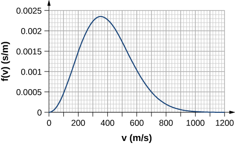
About 0.072. Answers may vary slightly. A more accurate respond is 0.074.

Using a numerical integration method such as Simpson's rule, find the fraction of molecules in a sample of oxygen gas at a temperature of 250 K that have speeds betwixt 100 m/s and 150 1000/south. The molar mass of oxygen $\left({\text{O}}_{2}\right)$ is 32.0 m/mol. A precision to two significant digits is enough.

Find (a) the nearly likely speed, (b) the average speed, and (c) the rms speed for nitrogen molecules at 295 K.

a. 419 m/s; b. 472 thou/south; c. 513 1000/south

Repeat the preceding problem for nitrogen molecules at 2950 Thou.

At what temperature is the average speed of carbon dioxide molecules $\left(M=44.0\phantom{\rule{0.2em}{0ex}}\text{g/mol}\right)$ 510 m/s?

541 M

The most probable speed for molecules of a gas at 296 Thousand is 263 g/southward. What is the tooth mass of the gas? (You lot might like to figure out what the gas is likely to exist.)

a) At what temperature exercise oxygen molecules have the aforementioned average speed as helium atoms $\left(M=4.00\phantom{\rule{0.2em}{0ex}}\text{g/mol}\right)$ have at 300 K? b) What is the answer to the same question about most probable speeds? c) What is the answer to the same question about rms speeds?

2400 K for all iii parts

Additional Problems

In the deep space between galaxies, the density of molecules (which are mostly single atoms) can be as depression as ${10}^{6}\phantom{\rule{0.2em}{0ex}}{\text{atoms/m}}^{3},$ and the temperature is a frigid 2.7 K. What is the pressure? (b) What volume (in ${\text{m}}^{3}$ ) is occupied by one mol of gas? (c) If this volume is a cube, what is the length of its sides in kilometers?

The air inside a hot-air balloon has a temperature of 370 K and a pressure level of 101.3 kPa, the same every bit that of the air outside. Using the composition of air as $78\text{%}\phantom{\rule{0.2em}{0ex}}{\text{N}}_{2},21\text{%}{\text{O}}_{2},\phantom{\rule{0.2em}{0ex}}\text{and}\phantom{\rule{0.2em}{0ex}}1\text{%}\phantom{\rule{0.2em}{0ex}}\text{Ar}$ , find the density of the air inside the airship.

When an air chimera rises from the lesser to the top of a freshwater lake, its volume increases by $80%$ . If the temperatures at the bottom and the peak of the lake are 4.0 and 10 $\text{°}\text{C}$ , respectively, how deep is the lake?

seven.9 m

On a warm day when the air temperature is $30\phantom{\rule{0.2em}{0ex}}\text{°C}$ , a metal tin can is slowly cooled by adding bits of ice to liquid water in information technology. Condensation starting time appears when the can reaches $15\phantom{\rule{0.2em}{0ex}}\text{°C}$ . What is the relative humidity of the air?

$40.18%$

The mean free path for helium at a sure temperature and pressure is $2.10\phantom{\rule{0.2em}{0ex}}×\phantom{\rule{0.2em}{0ex}}{10}^{-7}\phantom{\rule{0.2em}{0ex}}\text{m}\text{.}$ The radius of a helium cantlet tin can be taken as $1.10\phantom{\rule{0.2em}{0ex}}×\phantom{\rule{0.2em}{0ex}}{10}^{-11}\phantom{\rule{0.2em}{0ex}}\text{m}$ . What is the measure of the density of helium nether those conditions (a) in molecules per cubic meter and (b) in moles per cubic meter?

a. $2.21\phantom{\rule{0.2em}{0ex}}×\phantom{\rule{0.2em}{0ex}}{10}^{27}\phantom{\rule{0.2em}{0ex}}{\text{molecules/m}}^{3};$ b. $3.67\phantom{\rule{0.2em}{0ex}}×\phantom{\rule{0.2em}{0ex}}{10}^{3}\phantom{\rule{0.2em}{0ex}}{\text{mol/m}}^{3}$

The mean gratuitous path for methane at a temperature of 269 K and a pressure of $1.11\phantom{\rule{0.2em}{0ex}}×\phantom{\rule{0.2em}{0ex}}{10}^{5}\phantom{\rule{0.2em}{0ex}}\text{Pa}$ is $4.81\phantom{\rule{0.2em}{0ex}}×\phantom{\rule{0.2em}{0ex}}{10}^{-8}\phantom{\rule{0.2em}{0ex}}\text{m}\text{.}$ Find the effective radius r of the methane molecule.

In the chapter on fluid mechanics, Bernoulli's equation for the period of incompressible fluids was explained in terms of changes affecting a pocket-sized volume dV of fluid. Such volumes are a primal thought in the study of the flow of compressible fluids such as gases likewise. For the equations of hydrodynamics to utilize, the mean gratis path must be much less than the linear size of such a volume, $a\approx d{V}^{1\text{/}3}.$ For air in the stratosphere at a temperature of 220 Grand and a pressure of 5.eight kPa, how big should a be for it to exist 100 times the mean complimentary path? Take the effective radius of air molecules to be $1.88\phantom{\rule{0.2em}{0ex}}×\phantom{\rule{0.2em}{0ex}}{10}^{-11}\phantom{\rule{0.2em}{0ex}}\text{m},$ which is roughly right for ${\text{N}}_{2}$ .

eight.ii mm

Notice the total number of collisions between molecules in 1.00 south in 1.00 50 of nitrogen gas at standard temperature and pressure ( $0\phantom{\rule{0.2em}{0ex}}\text{°C}$ , i.00 atm). Use $1.88\phantom{\rule{0.2em}{0ex}}×\phantom{\rule{0.2em}{0ex}}{10}^{-10}\phantom{\rule{0.2em}{0ex}}\text{m}$ equally the effective radius of a nitrogen molecule. (The number of collisions per second is the reciprocal of the collision time.) Keep in mind that each standoff involves two molecules, so if one molecule collides once in a certain period of fourth dimension, the collision of the molecule it hit cannot exist counted.

(a) Gauge the specific oestrus chapters of sodium from the Law of Dulong and Petit. The molar mass of sodium is 23.0 chiliad/mol. (b) What is the percent mistake of your estimate from the known value, $1230\phantom{\rule{0.2em}{0ex}}\text{J/kg}\phantom{\rule{0.2em}{0ex}}·\text{°}\text{C}$ ?

a. $1080\phantom{\rule{0.2em}{0ex}}\text{J/kg}\phantom{\rule{0.2em}{0ex}}\text{°C}$ ; b. $12%$

A sealed, perfectly insulated container contains 0.630 mol of air at $20.0\phantom{\rule{0.2em}{0ex}}\text{°C}$ and an iron stirring bar of mass 40.0 g. The stirring bar is magnetically driven to a kinetic energy of 50.0 J and allowed to tedious down past air resistance. What is the equilibrium temperature?

Observe the ratio $f\left({v}_{\text{p}}\right)\text{/}f\left({v}_{\text{rms}}\right)$ for hydrogen gas $\left(M=2.02\phantom{\rule{0.2em}{0ex}}\text{g/mol}\right)$ at a temperature of 77.0 One thousand.

$2\sqrt{e}\text{/}3$ or nearly 1.10

Unreasonable results. (a) Find the temperature of 0.360 kg of water, modeled as an ideal gas, at a pressure of $1.01\phantom{\rule{0.2em}{0ex}}×\phantom{\rule{0.2em}{0ex}}{10}^{5}\phantom{\rule{0.2em}{0ex}}\text{Pa}$ if it has a volume of $0.615\phantom{\rule{0.2em}{0ex}}{\text{m}}^{3}$ . (b) What is unreasonable about this answer? How could yous go a better answer?

Unreasonable results. (a) Discover the average speed of hydrogen sulfide, ${\text{H}}_{2}\text{S}$ , molecules at a temperature of 250 Thou. Its molar mass is 31.iv g/mol (b) The result isn't very unreasonable, but why is it less reliable than those for, say, neon or nitrogen?

a. 411 k/s; b. According to (Figure), the ${C}_{V}$ of ${\text{H}}_{2}\text{S}$ is significantly different from the theoretical value, so the ideal gas model does not describe it very well at room temperature and pressure, and the Maxwell-Boltzmann speed distribution for ideal gases may not concord very well, even less well at a lower temperature.

Challenge Issues

An closed dispenser for drinking water is $25\phantom{\rule{0.2em}{0ex}}\text{cm}\phantom{\rule{0.2em}{0ex}}×\phantom{\rule{0.2em}{0ex}}10\phantom{\rule{0.2em}{0ex}}\text{cm}$ in horizontal dimensions and 20 cm tall. Information technology has a tap of negligible book that opens at the level of the bottom of the dispenser. Initially, information technology contains water to a level 3.0 cm from the height and air at the ambient pressure, 1.00 atm, from there to the top. When the tap is opened, h2o will flow out until the estimate pressure level at the bottom of the dispenser, and thus at the opening of the tap, is 0. What volume of water flows out? Presume the temperature is constant, the dispenser is perfectly rigid, and the water has a constant density of $1000\phantom{\rule{0.2em}{0ex}}{\text{kg/m}}^{3}$ .

8 bumper cars, each with a mass of 322 kg, are running in a room 21.0 one thousand long and 13.0 thou wide. They have no drivers, so they simply bounce effectually on their own. The rms speed of the cars is 2.fifty thou/s. Repeating the arguments of Force per unit area, Temperature, and RMS Speed, find the average forcefulness per unit length (analogous to force per unit area) that the cars exert on the walls.

29.five N/k

Verify that ${v}_{p}=\sqrt{\frac{2{k}_{\text{B}}T}{m}}$ .

Verify the normalization equation ${\int }_{0}^{\infty }f\left(v\right)dv=1.$ In doing the integral, offset make the substitution $u=\sqrt{\frac{m}{2{k}_{\text{B}}T}}v=\frac{v}{{v}_{p}}.$ This "scaling" transformation gives yous all features of the respond except for the integral, which is a dimensionless numerical factor. You'll need the formula

${\int }_{0}^{\infty }{x}^{2}{e}^{\text{−}{x}^{2}}dx=\frac{\sqrt{\pi }}{4}$

to find the numerical factor and verify the normalization.

Substituting $v=\sqrt{\frac{2{k}_{\text{B}}T}{m}}u$ and $dv=\sqrt{\frac{2{k}_{\text{B}}T}{m}}du$ gives
$\begin{array}{cc}{\int }_{0}^{\infty }\frac{4}{\sqrt{\pi }}{\left(\frac{m}{2{k}_{\text{B}}T}\right)}^{3\text{/}2}{v}^{2}{e}^{\text{−}m{v}^{2}\text{/}2{k}_{\text{B}}T}dv\hfill & ={\int }_{0}^{\infty }\frac{4}{\sqrt{\pi }}{\left(\frac{m}{2{k}_{\text{B}}T}\right)}^{3\text{/}2}\left(\frac{2{k}_{\text{B}}T}{m}\right){u}^{2}{e}^{\text{−}{u}^{2}}\sqrt{\frac{2{k}_{\text{B}}T}{m}}du\hfill \\ & ={\int }_{0}^{\infty }\frac{4}{\sqrt{\pi }}{u}^{2}{e}^{\text{−}{u}^{2}}du=\frac{4}{\sqrt{\pi }}\phantom{\rule{0.2em}{0ex}}\frac{\sqrt{\pi }}{4}=1\hfill \end{array}$

Verify that $\overline{v}=\sqrt{\frac{8}{\pi }\phantom{\rule{0.2em}{0ex}}\frac{{k}_{\text{B}}T}{m}.}$ Make the same scaling transformation as in the preceding problem.

Glossary

Maxwell-Boltzmann distribution: function that can exist integrated to give the probability of finding ideal gas molecules with speeds in the range between the limits of integration

most probable speed: speed near which the speeds of virtually molecules are establish, the peak of the speed distribution role

height speed: same as "most probable speed"

daigletheryiewer92.blogspot.com

Source: https://opentextbc.ca/universityphysicsv2openstax/chapter/distribution-of-molecular-speeds/

how do the speeds v1 and v2 compare to v0? that is, what are the ratios v1 v0 and v2 v0 ?

12 Distribution of Molecular Speeds

Learning Objectives

The Maxwell-Boltzmann Distribution

Summary

Conceptual Questions

Problems

Additional Problems

Challenge Issues

Glossary

0 Response to "how do the speeds v1 and v2 compare to v0? that is, what are the ratios v1 v0 and v2 v0 ?"

Postar um comentário

Iklan Atas Artikel

Iklan Tengah Artikel 1

Iklan Tengah Artikel 2

Iklan Bawah Artikel